LOOK FOR EXERCISE 2 SPECIFICATIONS COMING SOON. CLICK HERE! DON'T USE THIS ONE JUST YET!
 

READINGS

GUIDE 1: ISSUES IN MODELING GUIDE 2: TERMINLOGY GUIDE 3: THE LOWLY 2 X 2 TABLE GUIDE 4: BASICS ON FITTING MODELS GUIDE 5: SOME REVIEW, EXTENSIONS, LOGITS GUIDE 6: LOGLINEAR & LOGIT MODELS GUIDE 7: LOG-ODDS AND MEASURES OF FIT GUIDE 8: LOGITS,LAMBDAS & OTHER GENERAL THOUGHTS

OVERVIEW

 
 

KEY TAKEAWAYS A loglinear model is a set of created parameters that generates a [multivariate] table of expected cross tabulation cell frequencies The parameters in the equations for a loglinear model specify the marginal splits, associations and interactions on univariate, bivariate and multivariate cross tab tables. Before running statistical programs for your data, I suggest constructing a k-way percentage table IF feasible (it may not be past four variables) See if the table suggests possible associations and interactions among variables Note the two main abbreviated terminology ways to describe models Hierarchical models are easier to describe and test than non-hierarchical models However, sometimes a study design (e.g., an experiment) or a "structural zero" (e.g., pregnant men) invalidate a hierarchical model We use the likelihood ratio Chi-square statistic to measure model fit Sometimes we use L2 or G2 to describe the likelihood ratio Chi-square (the G indicates the general cell frequency model) This is a logged measure; we can "partition it" With this measure, we can compare two nested models (their G2 and df) to see if they differ beyond a chance level We view alpha levels and size differently for model fit here Remember: BIG chi-squares are BAD LITTLE chi-squares are GOOD Little chi-squares mean the modeled data well fits the observed data. This means we may be able to drop parameters for a simpler model (that's usually good and elegant) We test by dropping effects (e.g., a thre way interaction) and seeing if the G2 increases beyond a chance level To this point, I am describing a GENERAL CELL FREQUENCY loglinear model (GCF) The "dependent variable" is an interior cell frequency The "taus" are the multiplicative parameter estimates for the GCF The "lambdas" are the logged additive parameter estimates for the GCF (NOTE: the logits are from combinations of the lambdas and the betas are the logit coefficients you may remember from binomial logistic regression)

 

A QUICK WAY TO DESCRIBE A MODEL

As models contain more and more variables, it becomes increasingly difficult to describe them by providing an "illustrative table". Four variable tables are difficult enough to present. An example of a four variable table is below. I added study year (2014:2006) as a further control variable to the gender-education effects on the science question, and used percentages instead of cell frequencies (by each column) to this example to make the data slightly easier to read. as you can see, some of the cell sizes become small.

n = 1723

n = 2889

Source: NSF Surveys of Public Understanding of Science and Technology, 2006 and 2014. Director, General Social Survey (NORC).
 
 

BRIEF INTERPRETATION: Pause to consider. In 2006. both college and non-college men more often give the correct answer than comparably educated women, and to about the same relative degree. In 2014, the knowledge gap between men and women with under a college degree widens; the difference among college graduates reverses, with women scoring slightly higher than men. This interaction effect  is also suggested by the tau-betas for each of the four subtables: the same for both sexes in 2006 but quite different for 2014. (Try describing the taus in words!) But--is this just a chance fluxuation? Read on to find out.

Even with using percentages instead of cell frequencies, the tables become difficult to read. Tables with five or more variables typically confuse more than they clarify.
 

There are two common terminologies.

The first was briefly introduced in Guide Three and uses brackets. Where A, B, C and D refer to particular variables, we can sum up a model with all effects as simply:

if model {ABCD} is what is called a hierarchical model, the terms look like those in the table.Stay tuned, we will have more shortly on hierarchical models.
A model is hierarchical if all lower order terms are contained within the model abbreviation. For our four variable generic model, the hierarchical model {ABCD} would include:
 

As you can see, it is far easier to summarize a hierarchical model with just the highest term(s) in brackets.
 

If we decide that the model that is the simplest and best describes the data is one that (to continue with the four variable case) includes only all three-way interactions and all lower terms, we can describe that hierarchical model briefly and summarized as follows:

This model would ensure that the modelled and observed:

• three-way interactions (all 4 of them),
• two-way associations (all 6 of them),
• one variable marginals (4 of these)
• and n were identical,

A hierarchical model that fixed the  {ABC}{ABD} three way interactions as well as the two-way {CD} interaction would be represented by:

Gilbert and some others use a related terminology with parentheses and asterisks instead. Using his terminology, the four-way hierarchical model would be:

The second hierarchical model with all three-way terms would be: (A*B*C)(A*B*D)(A*C*D)(B*C*D)

And the third, even simpler, hierarchical model corresponding to the {  } terminology above would be: (A*B*C)(A*B*D)(C*D)

Either set of terms is generally recognized by loglinear analysts. 

When we have hierarchical models, the observed data (and typically the modelled data) generally depart from equiprobability on the two way associations and in the univariate marginals. Thus, the summated terminology above does a good and simple job for many tables.

However, there are several occasions when models are not hierarchical. Then, not only must you describe every modelled parameter in the table with your terminology (see the descriptive table above for all the terms you would include for a four-variable table...) but you also should use particular statistical programs (more on these in the future) that allow you to model non-hierarchical tables, and in these circumstances, you must be certain to provide every single term you plan to model in your computer program input. Very strange things happen with your computer output, especially with SPSS,  if you don't include all the relevant terms when you specify the model, such as negative chi-squares.

Many of the logistic regression programs assume that your model is hierarchical. They won't tell you that, but that's the assumption behind the statistics they present and the degrees of freedom that they calculate. If you have a NON hierarchical model, logistic regression may be a bad choice.

Below are a couple of instances that could create non-hierarchical tables. In each case, these approximate what Gilbert calls "stratified sampling designs."

EXPERIMENTAL DESIGNS. It is very common in experimental designs to create treatment groups that are all the same size. In part, this dates back to before modern high speed computer programs when it was faster and easier to do hand calculations using Analysis of Variance if all the treatment groups were the same size.

For example, suppose your dependent variable was success rates at quitting smoking (cigarettes) using two treatment groups (nicotine gum, nicotine patch) and a control group that did not receive a nicotine supplement. You also wanted to see if gender influenced quit rates, either alone or in conjunction with a nicotine supplement. Thus you created the following study design. The cell frequencies are the planned number of cases in each treatment
 
 

As you can see if you calculate the marginals (and even if you don't and just stare at the table), the gender marginal, the treatment marginal and the gender by treatment experimental associations will all be equiprobable (and do not need to be modelled) because of the experimental design. However, higher order terms (perhaps a gender by treatment by cessation rate interaction effect) might NOT be equiprobable.

  DISPROPORTIONATE SAMPLING DESIGNS. We select cases with disproportionate probabilities typically when we have some small subgroups and wish to have enough cases from that subgroup so that our inference tests have sufficient statistical power. Recall that any sample design in which each element has a known and non-zero chance of selection is a probability sample. Thus, disproportionate designs are very often   probability samples. However, we have often oversampled some groups and undersampled others compared with sampling probability proportionate to size or "self weighted" samples.

For example, when we look at the science question X gender X degree level X (now added) ethnicity table in the observed SDA data in the General Social Survey, 2014 NonWhite respondents are far outnumbered by White respondents in the USA. Currently, Whites comprise a bit over 75 percent of adult GSS survey respondents (1885/2535 in 2014). The smaller numbers of NonWhite respondents can present analytic problems when we wish to further subdivide the table, e.g., by gender and degree level. Thus, were we to create a new study, we may wish to overselect African-Americans, Hispanic-Americans, and Asian-Americans, the groups most prevalent in the U.S. (keeping in mind that Hispanics could be of White, African or Asian descent, thus adding yet another possible dimension to our sampling design).

One example could be:

Because of the sampling scheme in the table above, there will be no association between gender and ethnicity, between gender and degree level, or between ethnicity and degree level in the observed tables. However, there could be higher order interactions among gender, ethnicity, degree level and a dependent variable, such as the planetary question. Hence, this is a non-hierarchical model.

Hopefully no one has any problems seeing why the planetary question would be the dependent variable. But if you do have problems here, please review the material on causality in Guide 1.

PEARSON CHI-SQUARES AND (LOG) LIKELIHOOD-RATIO CHI-SQUARES

One of the big advantages that loglinear models have over more traditional ways of examining multivariate tables is the use of tests of statistical significance to test whether interaction effects and partial association (controlling other variables) effects are zero or are greater than zero. Being able to use these multivariate tests of statistical significance is one of the features that turns loglinear modelling into a system, comparable to N-way analysis of variance or multiple regression instead of the physical control and inspection of separate partial crosstabulation tables I demonstrated earlier this semester.

In a later guide we will see that we can also ascertain whether certain effects can be dropped or should be retained by examining the specific Z-scores related to effect parameters.

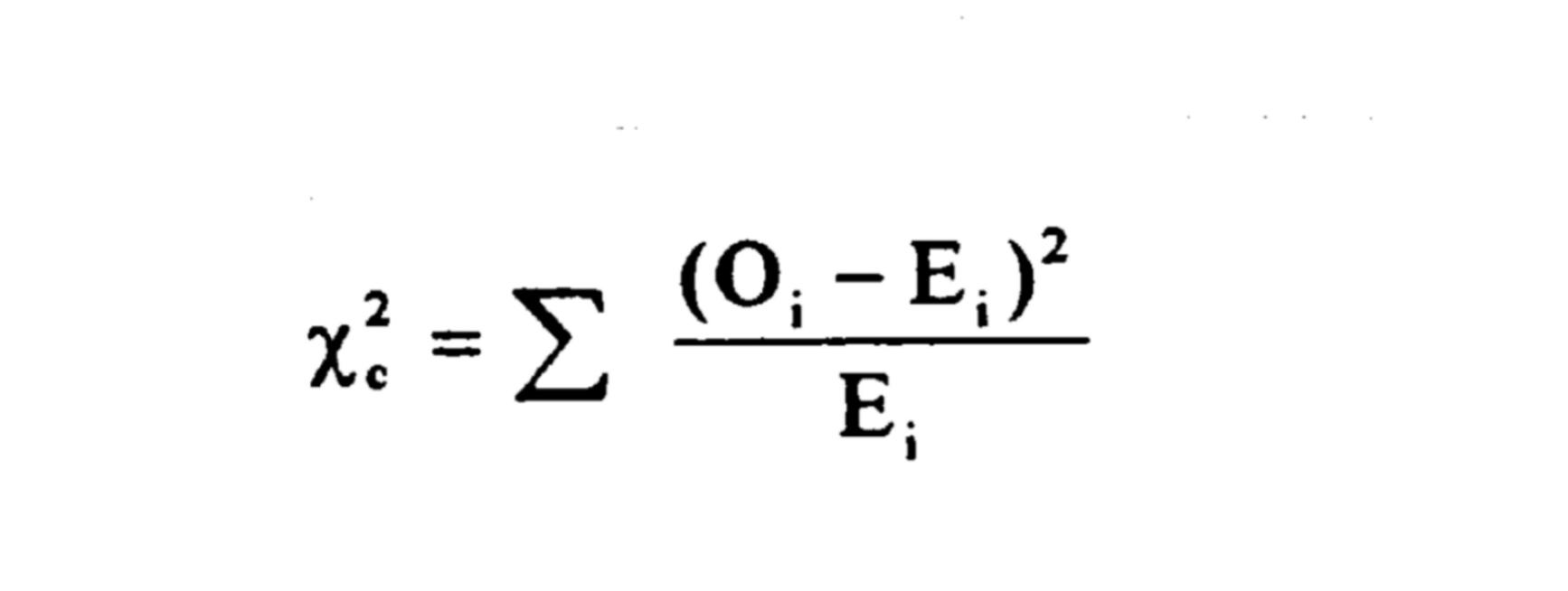
The formula for the traditional Pearson Chi-Square statistic is repeated below. This is the same formula presented in Guide 3. Notice that this is a multiplicative formula because in each term, we divide by the modelled or expected frequency for a particular cell.

Instead of the Pearson Chi-Square, testing in loglinear analysis uses the likelihood ratio Chi-Square statistic (sometimes called the log likelihood ratio statistic due to the logged terms in the formula). One version of the formula for the likelihood ratio Chi-square statistic is given immediately below:

Where ln x_ij is the natural log of the OBSERVED  cell frequency.
Where  ln m_ij is the natural log of the MODEL or EXPECTED cell frequency.

[NOTE: I sometimes call this L² (that's another version).]  As you can see, the likelihood ratio chi-square statistic and the Pearson (multiplicative) chi-square statistic are relatives. In large (estimated over 100) samples, they both have a Chi-square distribution and can use the Chi-square tables. The calculated values are also quite similar in very large (bigger than n = 100!) samples but are not necessarily so in small samples. 

The biggest advantage of the likelihood ratio statistic is that it is additive. That means that G² can be partitioned and portions of the statistic allocated to different pieces of a particular model.

However, the G²  statistic can only be partitioned for nested models. A model can be said to be nested if the more complex model contains ALL the terms of a simpler, lower order model (and more terms than the simpler model besides).

For example, the hierarchical model (A*B*C) contains the three way interaction, the three two way associations, and the three marginal terms (as well as the case base, which we can assume is a typical feature in virtually all loglinear models).

Thus the hierarchical model: (A*B)(A*C)(B*C) "is nested" in the more complex model (A*B*C) because the model (A*B*C) contains every term that is in the model (A*B)(A*C)(B*C) as well as the additional three variable interaction effect A*B*C.

We can subtract the G² for the more complex model from the G² for the simpler model. (The simpler model has a bigger G² than the more complex model with more terms.)

We can also subtract the corresponding degrees of freedom (The simpler model has more df reflecting the terms that are not "fixed."). That result is ALSO distributed as a G² with df equal to the difference in degrees of freedom between the two models.

The chi-square statistic for simpler nested models is virtually always larger than the chi-square statistic for more complex models. This is because the more complex model has more parameters, and hence the expected and observed cell frequencies are a better match and the chi-square statistic (and fewer df because we "fixed" more parameters) is smaller than it is for simpler models.

Similarly, the more complex model has fewer degrees of freedom than the simpler model. Because the more complex model has to fit more marginals, associations, and interaction effect, it "uses up" more degrees of freedom than the simpler model, with fewer parameters to estimate, does.

Using the four way table above for the 2014 and 2006 NSF Surveys with the planetary question, gender and education, I test models in the section below. But to anticipate briefly:

A hierarchical saturated model that includes the four variable interaction has a G² of 0 and 0 degrees of freedom (as saturated models always do).

MODEL A: A hierarchical model that omits the four variable interaction has 1 degree of freedom (because this is a special case where all the variables have only two categories or values) and a G² of 3.23 (p = 0.072).

MODEL B: A hierarchical model that omits the four variable interaction and also the three way possible association among gender, year and degree level has 2 degrees of freedom (we gain back another df by omitting the gender by year by degree three way association--each variable again has only two values) and a G² of 5.15 (p = 0.076). The  difference between Model B - Model A is a likelihood ratio statistic G² of:  5.15 - 3.23 = 1.92 with 2 - 1 or 1 df.

In my example, the difference between the two models falls far short of statistical significance but that is not always the case. Partitioning the G² may enable us to see exactly where the important parameters of a complex model lie.

As we will shortly see, neither of these two models presents a "good fit" to the data.

You can ONLY use the G² partitioning for nested models. You cannot use it to compare two models that are not nested.
For example, you could not subtract the G²s and their associated degrees of freedom for the following two models:

{AB}          versus          {BC}

The {AB} model which contains AB, A and B versus
the {BC} model which contains BC, B and C

{AB} and {BC} are not subsets of each other. The first model contains the A marginal which is nowhere to be found in the second model and the second model contains the C marginal which is nowhere to be found in the first model. So you cannot subtract either the G²s  or the degrees of freedom.
 
 

Both in the case of evaluating an overall G²  for a model, or assessing the G²  difference for two nested models, we tend to enlarge the alpha level. Partly this is to depress levels of type 2 error which many computer programs do not calculate. For the same size n, an increase in the type 1 error level tends to decrease the probability of a type 2 error (although note that this is not an exact inverse relationship especially with large samples).

In addition, our preference is to go with simpler models that contain fewer parameters to describe the data when this is possible.

Thus, in loglinear analysis, to assess a model overall, or to test the differences across nested models, we tend to adopt a 0.20 type 1, , or probability level MINIMUM. This implies that we will not add additional parameters to describe the model unless it is absolutely necessary.

BASIC MODEL TESTING

 

During model testing, we compare the generated [modeled, expected] cell frequencies with the observed frequencies. If the two sets overall are within sampling error of one other, as it was with each of my Models 1 and 2 above, "the simpler [leaner] model fits".

If the deviations between the two are beyond sampling error, that model is a "poor fit". When the fit is poor, we usually add back parameters that generate new expected or modeled frequencies that are closer on the average to the real or observed frequencies that create a "better fit".

We test the fit of a particular model with a likelihood ratio Chi-square statistic. Large G²s mean large deviations between the modeled and observed data, and this means that the model "doesn't fit". Parameters must be added to the model equation (see below) so that the modeled and observed frequencies become more similar to one another. The most complex model, the fully saturated model, generates expected frequencies that exactly match the observed frequencies. Thus, the fully saturated model always "fits perfectly" and the G²s is 0. Most of the time, however, the saturated model is not considered "very interesting."

The parameters in the equations for a loglinear model specify the marginal splits, associations and interactions on univariate, bivariate and multivariate cross tab tables. For example, one important set of parameters creates the "independence model". Here's what you used to do with the typical 2 X 2 cross tabulation table: in the independence model for a two way table, you selected parameters such that the total case base and both univariate marginal distributions exactly matched the observed data. That is, you allow the univariate odds-ratios to depart from 1 if that is the case in the real dataset.

However in the classic "independence model" the second order odds was set to 1 (ln odds = 0).  This forces the relative frequency distribution (percents or proportions) on the second variable to be the same across each category of the first variable and to match the univariate marginal (e.g., we would set about 20 percent of both men and women to give the wrong answer on the planetary question if this were the total sample percent as shown in Guide 3). You then compared the expected frequencies generated under the independence model with the observed frequencies. With a large X², you rejected the independence model. The parameter that specified a relationship between the two variables (i.e., made the modelled cells match the observed cells) had to be returned to the model.

This addition of the final 2 way parameter created a second order interaction (association) between the two variables, a subsequent saturated model with a G² = 0 and 0 df.
 

We follow a similar pattern of model testing with more complex tables. It is a good idea to first write down the fully saturated model (e.g., {ABCD} in the four variable case below) so that you know what all the model parameters are. That way you will have an idea of which effects to eliminate first.

Here I am assuming a hierarchical model unless I mention otherwise.

It's a very good idea to write down all the desired parameters FIRST, before you specify the SPSS computer model.

Then, OMIT the effect from the model that you wish to test and observe the G² statistic. If the G²  is very large relative to the degrees of freedom, the specified model does not fit. The omitted parameter must be returned to the model to make the observed and expected cell frequencies match within sampling error.

On the other hand, if the simpler model fits, see what additional parameters can also be dropped. You can assess the new model both overall, and also compare it via  partition to a more complex model in which the new model is nested.

In the planetary question by gender by degree level by year table, we begin with 16 cells and 16 df. We have four marginals (each, in this case, subtracts [2 - 1] X 4 or a total of 4 df), four three way effects (lose another 4 df), six two way effects (also "eating" 6 df), a possible four way interaction effect (1 df) and the case base (the last df) in the fully saturated model.

The very first table above is presented in terms of percentages.

(NOTE: I recommend this when you begin working with tables; it helps you interpret your results and may suggest models that are simpler than the saturated model.)

When we examine those percentages in the very first four way table, we see that first, regardless of gender, better educated individuals more often get the question right. Second, within each level of education except for the high degree group only in 2014, men more often give the correct answer than women do. These are "joint" effects, both independent variables (gender and degree) overall influence the response variable or planetary question.

Third, there MAY be an interaction among year, gender, education, and the planetary question. Gender seems to make more of a difference in 2014 especially in obtaining the right answer among the less educated respondents than it does among the better educated respondents. However, this apparent interaction effect could simply be sampling error. A total sample of 2889 is a nice size, to be sure, but notice that each of the separate educational subtables is smaller than that total n. (The application of the GSS sample weights will cause small variations in the case base from analysis to analysis.)

In terms of the loglinear equations below, where A = year, B = gender, C = degree level and D = planetary question response, we could describe the saturated model this way:

G_ijk =  + _i^A + _j^B +_k^C + _l^D + _ij^AB + _ik^AC + _il^AD + _jk^BC + _jl^BD + _kl^CD + _ijk^ABC_ijl^ABD +_ikl^ACD + _jkl^BCD + _ijkl^ABCD

In a further guide, we will discuss the lambda numeric parameters in the equation. Note here that these are additive parameters because the s are logged from the original multiplicative equations.

Using abbreviated model notation, either set of terms below would also describe this saturated hierarchical model:

{ABCD}
(A*B*C*D)

BASIC LOGLINEAR EQUATIONS

The loglinear model we have been working up until now with is often called the General Cell Frequency Model (GCF)

In the GCF model, we are trying to predict or model a cell frequency. Cell frequencies can be created by marginal splits (in a 1 by k table), two variable cross-tabulations, cross tabulating two variables within categories of a third and so forth.

Of all the models we consider this semester, the GCF model allows  the most flexibility. We readily observe all associations, including those among independent variables. We can test "path-like" causal models (I will draw some in class), check for indirect causal effects and statistical interactions (specifications) more readily in GCF models than in other kinds of models, e.g., logit models or logistic regression.

Predictors that have an effect (are statistically significant) in GCF models raise or lower the predicted cell frequencies (F_ij in the original multiplicative model and ln F_ij = "Gij" in the logged additive and linear model) in a multivariate crosstabs table. Negative (logged)  Gij parameters mean fewer frequencies in a cell than would occur with a predicted equiprobable or no effect model. Positive (logged)  Gij parameters parameters mean more frequencies in a cell than an equiprobable or no effect model would predict.
 

The original formula that produces the cell frequency is multiplicative (think back to the probabilities divided by the case base in Guide 3).

A   X B  X C   X  n

for a three variable A by B by C table.

More formally, we write out the loglinear equation as a set of parameters using eta for the "grand mean" (the equiprobable model) and taus for the variables and combinations of variables. For example, for three variables, A, B and C, the formula for the fully saturated loglinear model is given below. This is a multiplicative model that predicts the literal cell frequencies (not in logged form)  F_ijk.

EQUATION 1:      F_ijk =  * _i^A * _j^B * k^C * _ij^AB * _ik^AC * _jk^BC * _ijk^ABC

recall that:          ln (A * B)  = ln A + ln B

and:                     ln (A/B)  = ln A - ln B

Multiplicative and nonlinear coefficients are generally more difficult to interpret than linear and additive parameter coefficients. By taking natural logarithms of both sides of Equation 1, we can create an additive and linear model equation in Equation 2, hence the term "loglinear". In the transformed model equation for the parameters, the ln F_ij are now called "Gij" and the new parameters are lambdas rather than taus. So Equation 1 now becomes:

EQUATION 2:      G_ijk =  + _i^A + _j^B + _k^C + _ij^AB + _ik^AC + _jk^BC + _ijk^ABC
 

The theta parameter (eta in the multiplicative model) is for the "grand mean" or "fixing n" in the equiprobable or simplest model.
 
 

In later guides, we will see how this equation can be transformed in the cases of logits or logistic regression. But make no mistake about it: what you see above in the loglinear basic equation is THE basic equation.

It is the foundation for logistic regression but it contains much more. The loglinear model allows you to simultaneously explore the relationship among possible independent variables (in the two variable associations) as well as possible indirect causal effects on a postulated dependent variable.

Equations 1 and 2 addressed the fully saturated model. However, our goal is to have the simplest possible model that fits the data with the fewest number of parameters. For example, if the independent variables are uncorrelated, these terms can be dropped from the model (e.g., _ij^AB  ). If a third order interaction (e.g.,_ijk^ABC ) is unnecessary, it can be dropped from the equation as well.

For example, the hierarchical model {AB}{AC} (which also contains the {A}{B} and {C} parameters) is written this way:

EXAMPLE MODEL:      G_ijk =  + _i^A + _j^B + _k^C + _ij^AB + _ik^AC

(We never specified a BC term so it is omitted from the equation above. )
 

READINGS

OVERVIEW

This page created with Netscape Composer
Susan Carol Losh
February 5 2017