|
KEY TAKEAWAYS
|
|
THE MULTIVARIATE ANALYSIS OF CATEGORICAL DATA GUIDE 3: THE "LOWLY" 2 X 2 TABLE (and a bit on three way tables too) Susan Carol Losh Department of Educational Psychology and Learning Systems Florida State University |
|
THINGS" |
AND 2 x 2 TABLES |
A THEME |
|
|
|
|
A statement you will increasingly see in both Gilbert and Agresti is about "fixing" parameters. They will discuss "fixing" the total case base or a marginal frequency distribution. Associations are often "fixed" as are often two way or higher interactions.
This is actually a relatively simple construct. Remember that we are creating an "imaginary world" when we create a statistical model. For example, one of the simplest possible models is called "the equiprobable model" where the frequency or count in a particular cell is the same for ALL the cells in the table. For a table containing the bivariate distribution of two binary variables, that is, a table with two rows and two columns (2 X 2), each expected cell frequency would be the same and equal the case base divided by the number of cells (here, four) or simply: n/4. In the equiprobable model, the row totals would be identical for each row; the column totals would be identical for each column, and the row totals would equal the column totals. In the equiprobable model, all the parameters have been created by the model--except one: the total case base.
We follow the convention, which occurs in virtually all such multivariate categorical models, that the model case base is set or "fixed" by the observed sample or population case base. In other words, the model parameter for the case base is identical, or "fixed", to the empirically observed case base.
Thus, to "fix" a model parameter is to constrain that parameter to equal the equivalent empirically observed parameter in the table. To "fix" the marginals means that the model parameters for the table marginals will exactly reproduce the observed table marginals. To "fix" a two-way association means that we require all four cells in our 2 X 2 model table to exactly replicate the observed empirical 2 X 2 table.
AND A BIT ON DEGREES OF FREEDOM AND FIXING PARAMETERS
Fixing parameters comes at "a price." By constraining some of the model parameters to equal the empirically observed paraments (such as row totals), we are taking a great role in dictating what the frequencies in the table will look like under the specified model. We will examine degrees of freedom in more depth later, but as a beginning:
The total degrees of freedom we begin with equals the total number of cells in the table.
In the 2 X 2 table, that is 4.If we constrain or "fix" the model case base to equal the empirically observed case base, we lose 1 degree of freedom (df) for n.But, remember in larger and multi-dimensional tables, we must multiply across ALL the variables and their values in the entire table. For example, in a 2 X 2 X 2 X 2 four-variable table, we would begin with a total of 16 cells and 16 degrees of freedom. In my perceived scientist agreement (3) by political party identification(3) by year, 2006, 2010 (2) we begin with 3 X 3 X 2 = 18 df.
If we require in a 2 X 2 table that the model row totals match the observed row totals, we lose i - 1 degrees of freedom, where i is the number of rows. It is i- 1 because if we know i - 1 row totals and we know n, we can obtain the last model row total by subtraction. (Thus, the ith row is called linearly dependent upon n and the first i-1 rows.)
If we require in a 2 X 2 table that the model column totals match the observed column totals, we lose another j - 1 degrees of freedom, where j is the number of columns. It is j - 1 because if we know j - 1 column totals and we know n, we can obtain the jth model column total by subtraction (linear dependence again).
Let's look at this from the viewpoint of "fixing" the n and the row and column totals: Start with 4 df for 4 cells in the table. |
|
|
Let's consider what we USED to do to see whether two variables were related or independent in cross-tabulation tables.
To say that two variables are related is to say that a change in the distribution of the first variable is associated with a systematic change in the distribution of the second variable.
To say that two variables are independent is to say that changes in the distribution of the first variable are not associated with (are independent of) any systematic change in the distribution of the second variable.
In odds ratio terms, the second order odds ratio equals 1 when two variables are independent. Put slightly differently, this means that the first order conditional odds for one variable are identical across categories of a second variable.
Since the logarithm of 1 for either natural logs or base 10 logs is 0, the log of the odds will be zero when two variables are independent.
In "Statistics 101" we typically tested whether there was a relationship between two variables by using the null hypothesis: X2 = 0, that the two variables were independent. If the probability of attaining the value of X2 that we observed (or larger) in our sample data was highly unlikely under the null hypothesis (e.g., p < .0001), we rejected the H0 of independence and went with the alternative, HA, that X2 was something greater than zero and that some relationship between the two variables existed. Notice, of course, that in rejecting the H0, we did not know what the value of X2 (or any associated correlation coefficient) was, we only knew what the value was not, i.e., zero.
Below is the formula that most of us were taught in introductory statistics to calculate Chi-square under the assumption of independence in bivariate distribution tables:
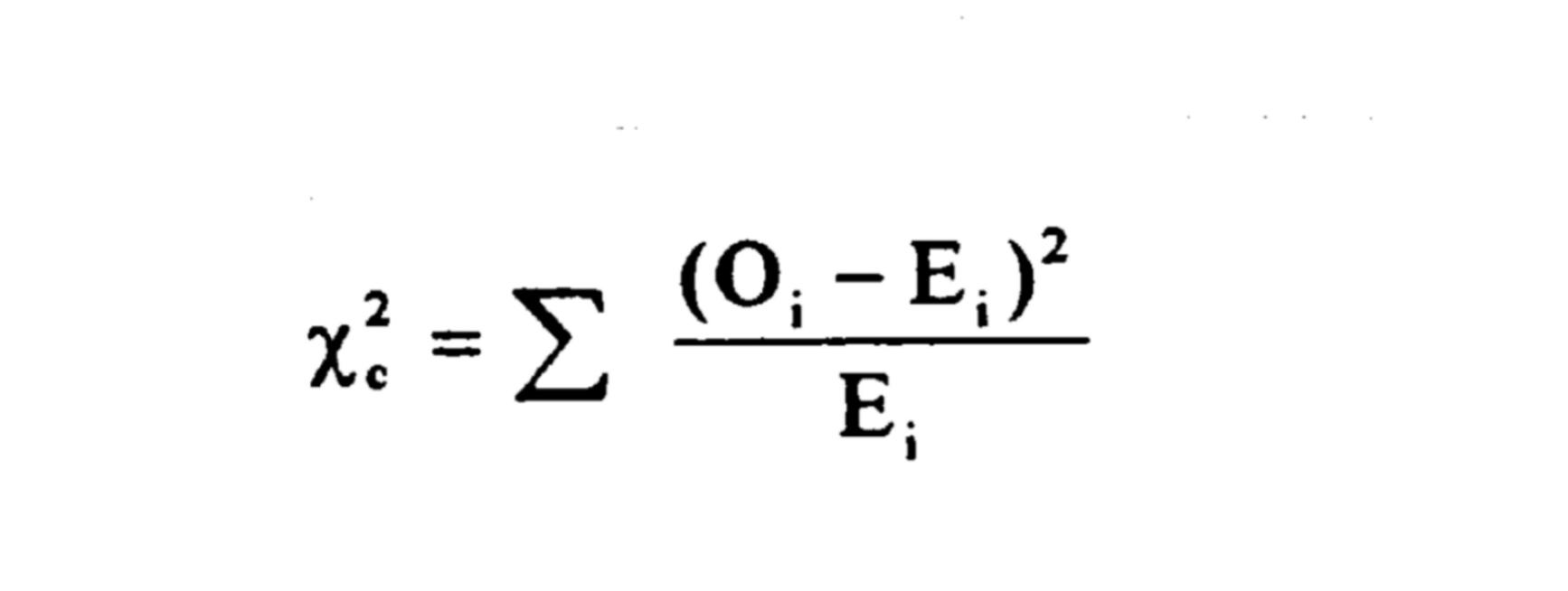
The "O" is the OBSERVED frequency in a specific cell, say, row 1 column 1. (O = Observed) The "E" is the EXPECTED frequency in the identical cell, say, row 1 column 1. (E = Expected)
Obviously the key to the Pearson X2
under
the null hypothesis is the difference between the empirically observed
sample values in the cross-tabulation table and the expected values under
the assumption of independence. As the difference between the observed
and expected values gets larger and larger, X2 becomes
larger and larger, and the model assumption of statistical independence
between two variables becomes more and more untenable. (If you use an SDA
cross tab, they colorfully code these cells in shades of red or blue.)
So a key to testing for independence is HOW we obtain these expected frequencies.
How do we obtain these "expected frequencies" that would occur if the correlation between two variables is zero? In the "Statistics 101 way," we obtained the expected frequencies are determined by multiplying selected marginals and dividing by the the sample size.
Let's take a look at the relationship between gender and the Earth and the Sun again.
Below are the OBSERVED FREQUENCIES:
| How Gender Influences Answers to the Question: Does the Sun go around the Earth or does the Earth go around the Sun? |
| Male | Female | Total | |
| Answer to Question: | |||
| Sun goes around Earth (WRONG and other responses except earth around sun) | 72
(r1, c1) |
165 | 237 |
| Earth goes around Sun (RIGHT) | 468 | 461 | 929 |
| Total (at the bottom of each column are SEPARATE totals for women and men, then a total for everyone combined) | 540 | 626 | 1166 |
Source: NSF Surveys of Public Understanding
of Science and Technology, 2014, Director, General Social Survey (NORC).
Total valid n = 1173; MD = 7
When we wanted to obtain the EXPECTED male-wrong answer cell, we multiplied the marginal total for men (540) by the marginal total for the wrong answer (237) then divided by the case base (1166) or:
540 X 237
= 109.75
1166
Once we obtained the first cell frequency in a 2 X 2 table, we obtained the other 3 cells interior to the table by subtraction from the marginals and case base.
For example, the expected female-wrong answer cell would simply be the marginal total for the wrong answer (237) minus the expected frequency in the male-wrong answer cell (109.75) or, for the female-wrong answer cell:
237 - 109.75 = 127.25
|
|
I would like us to pause for a minute and think about what we just did. Most of us memorized the way to obtain expected frequencies in a 2 X 2 table and we haven't thought much about it in YEARS.
But here's another way to think about it.
When we calculated the male-wrong answer cell, what we actually did was to multiply the probability of being male (male/total) by the probability of being wrong (wrong/total) by the case base, or letting:
![]() = probability
= probability
M = Male
W = Wrong answer and
n =
the case base
![]() M
X
M
X ![]() W X
n
W X
n
or:
540/1166 X 237/1166 X 1166 = 109.75
This leads us to a slightly different way of thinking about the calculations for the expected frequencies in a two-way table.
Below are the OBSERVED COLUMN PERCENTAGES
for
the gender by planetary science question. Notice I have added a column
for percents on the planets question for the total sample to the
far right:
| How Gender Influences Answers to the Question: Does the Sun go around the Earth or does the Earth go around the Sun? |
| OBSERVED PERCENTAGES | Male | Female | Total Sample |
|
Answer to Question:
|
|||
|
Sun goes around Earth
(and
other responses...) WRONG)
|
13.4%
|
26.3%
|
20.3%
|
|
Earth goes around Sun
(RIGHT)
|
86.6
|
73.7
|
79.7
|
|
100.0%
|
100.0%
|
100.0%
|
|
|
Casebases
|
540
|
626
|
1166 |
Source: NSF Surveys of Public Understanding
of Science and Technology, 2014, Director, General Social Survey (NORC).
Total valid n = 1173; MD = 7
In sample data, we often use percentages to estimate the population probabilities of being in a particular category of a designated variable. A sample percentage divided by 100 is a sample proportion and we often use these sample proportions as "stand-ins" to estimate the population probabilities in each category.
What would our imaginary world look like if the gender variable and answers to the science question were independent, that is, if there were NO ASSOCIATION between gender and the science question?
In our fledgling loglinear terminology, this would be equivalent to:
|
Independence Model |
| EXPECTEDPERCENTAGES | Male | Female | Total Sample |
|
Answer to Question:
|
|||
|
Sun goes around Earth
(WRONG)
|
20.3%
|
20.3%
|
20.3%
|
|
Earth goes around Sun
(RIGHT)
|
79.7
|
79.7
|
79.7
|
|
100.0%
|
100.0%
|
100.0%
|
|
|
Casebases
|
540
|
626
|
1166 |
Then, we can use our knowledge of the relationship
among frequencies, percentages, and proportions to turn the percentages
in each column back into EXPECTED FREQUENCIES.
NUTS
AND BOLTS: CALCULATING EXPECTED FREQUENCIES
For row 1 column 1, the expected percent of men giving the wrong answer is 20.3 and the expected proportion is .203.
Multiply the expected proportion of men giving the wrong answer by the total casebase FOR MEN ONLY:
.203 X 540 = 109.62
(Note there will be small differences from my first calculations for expected frequencies due to rounding errors.)
Notice once again that with a 2 X 2 table, I have to calculate the expected frequency for ONLY ONE CELL in the table. See the yellow cell in the table below. Because of the "fixed" or constrained marginal totals in the far right column and the bottom row, I can get the other three cells by subtraction. We use the OBSERVED ROW AND COLUMN TOTALS to calculate the EXPECTED CELL frequencies.
For example, the expected cell frequency for the number of women giving the wrong answer will be:
237 - 109.6 = 127.4 or
Total observed frequency giving wrong answer - expected frequency MEN giving wrong answer =
expected frequency WOMEN giving wrong answer 127.4
Be sure to distinguish among observed and expected frequencies in the "right places."
The expected cell frequency for the number of men giving the right answer will be:
540 -109.6 = 430.4 or
Total observed male casebase - expected frequency MEN giving wrong answer =
expected frequency MEN
giving right answer
| How Gender Influences Answers to the Question: Does the Sun go around the Earth or does the Earth go around the Sun? |
| The yellow cell is the only one we must calculate totally. The other cells are obtained through subtraction. |
| EXPECTED CELL FREQUENCIES | Male | Female | Total Sample |
|
Answer to Question:
|
|||
|
Sun goes around Earth
(WRONG)
|
109.6
|
127.4
|
237
|
|
Earth goes around Sun
(RIGHT)
|
430.4
|
498.6
|
929
|
|
Casebases
|
540
|
626
|
1166 |
And, again by subtraction, we find that the expected frequency of WOMEN giving the RIGHT answer = 498.6
Notice that I only had to calculate the expected frequency for ONE CELL (Male, Wrong) (the "yellow cell") out of the four cells in the table, then I could obtain the other three expected frequencies in the table by subtraction from the marginal totals.
This means I only have ONE "degree of freedom" in my 2 X 2 table, or one "independent" piece of information. Once the expected number of males giving the wrong answer is calculated, all the other three interior cells of the table are calculated through subtraction. This is consistent with the calculations for degrees of freedom in the earlier part of this guide.
Using both the expected and the observed frequencies for our gender by education table and the Chi-Square calculation formulation, here's the calculations:
We start with the row 1,1 cell, then
the 1,2 cell.
Thus, calculations are done for the first
(or top) row, left to right.
We proceed to the second row to calculate
the X2 component for each of the cells in turn, from left to
right.
We do NOT use the row or column
marginals in the Chi-Square formula, only the internal cells in the table
itself.
[ ( 72 - 109.6 )2÷109.6]
+
[ (165 - 127.4)2÷127.4]
+
[ (468 - 430.4)2÷430.4]
+
[ (461 - 498.6 )2÷498.6].
OR
[ ( - 37.6)2÷109.6] + [ (37.6)2 ÷127.4] +[ (37.6)2÷430.4] + [ - 37.6 )2 ÷498.6].
OR
[ ( 1413.76 )÷109.6] + [ (1413.76) ÷127.4] +[ (1413.76)÷430.4] + [ (1413.76 ) ÷498.6].
(Remember, the square of a negative number in arithmetic is a positive number.)
OR
12.90 + 11.10 + 3.28 + 2.84 = 30.12
Chi-square might be small, or it might be large, but Chi-square should ALWAYS be a positive number.
X2 (1) = 30.12
The (1) subscript means that there is ONE degree of freedom in the table. You must include this information for your reader (or you) to accurately assess the value of Chi-Square.
(The LR X2 (1) = 31.09. The Pearson X2 and the Likelihood Ratio X2 are often similar for simple tables when n is "large" but not necessarily when n is small.)
|
|
What you did in Statistics 101 was accurate enough, as far as it went. What you were not told was that "the independence model" was just one model among several that could have been used to characterize the 2 X 2 table.
What are some of those other models?
![]() (1)
The very simplest is the "equiprobable model." In this model, each
cell has the same frequency as each other cell. The expected frequency
is simply the case base divided by the total number of cells in the table.
We have "fixed" the case base and nothing else.
(1)
The very simplest is the "equiprobable model." In this model, each
cell has the same frequency as each other cell. The expected frequency
is simply the case base divided by the total number of cells in the table.
We have "fixed" the case base and nothing else.
In my gender by planetary question table, each cell would simply be 1166/4 or 291.5We would have 4 - 1 or 3 df.Or Fij = n/(r X c)
where r = the number of rows and c = the number of columns
![]() (2)
Next, we could fix the case base, constrain the expected row totals
to equal the observed row totals, but fix the column totals to be equiprobable.
This
means the column totals would simply be the case base divided by the number
of columns.
(2)
Next, we could fix the case base, constrain the expected row totals
to equal the observed row totals, but fix the column totals to be equiprobable.
This
means the column totals would simply be the case base divided by the number
of columns.
In my example, this would mean a "50-50" split on gender or 1166/2 or 583 males and 583 females.
Using these new row and column totals we could then go ahead and calculate the expected values in the cells using the formula:
![]() M
X
M
X ![]() W X
n
W X
n
using the NEW probabilities for the columns, i.e., that the number of men = the number of women.
We would have 4 - 1 - 1 or 2 df.
![]() (3)
In
a third possible model, we could fix the case base and the expected column
totals to equal the observed values but calculate the expected row totals
to be equiprobable. This would imply a 50-50 wrong answer-right answer
distribution on the planetary questions. Once again we could calculate
the expected cell frequencies using the formula:
(3)
In
a third possible model, we could fix the case base and the expected column
totals to equal the observed values but calculate the expected row totals
to be equiprobable. This would imply a 50-50 wrong answer-right answer
distribution on the planetary questions. Once again we could calculate
the expected cell frequencies using the formula:
![]() M
X
M
X ![]() W X
n using the new probabilities for the rows.
W X
n using the new probabilities for the rows.
Again, we would have 4 - 1 - 1 or 2 df.
![]() (4)
Then,
there is the by now familar independence model, wherein we fix the case
base, the row totals and the column totals to equal the observed corresponding
values and calculate the cells in the interior of the table.
(4)
Then,
there is the by now familar independence model, wherein we fix the case
base, the row totals and the column totals to equal the observed corresponding
values and calculate the cells in the interior of the table.
Thus we would have 4 - 1 - 1 - 1 or 1 df.
![]() (5)
JUST
ONE MORE MODEL (at least for a 2 X 2 table): what can possibly be left?
(5)
JUST
ONE MORE MODEL (at least for a 2 X 2 table): what can possibly be left?
OK, let's fix the case base, the row totals
and the column totals so that they equal the observed values.
Now, fix the cells so that the expected
frequencies equal the observed frequencies.
Your model will now exactly reproduce all observed frequencies in the cells, the marginals, and the total.
This is a very special model:
This model now has zero degrees of freedom. You lost
This model is called the saturated model.In saturated models, the imaginary and real worlds totally overlap; the expected and observed values are totally equivalent. Because the expected and observed values in each cell are the same, this model always has a Chi-square of zero and zero degrees of freedom.
For structural equation model "graduates," notice the similarity with the saturated model with 0 df that exactly reproduces the variance-covariance matrix (or correlation matrix for standardized variables).
The X2 statistics and degrees of freedom parameters hold for all saturated models, irrespective of the number of rows or columns, or the number of variables being analyzed. They are always zero in saturated models.
If we reject the independence model in the two way table, our only alternative left to describe the data is the saturated model.
It is very common to need a saturated model
in two way tables. As the number of variables grows, saturated models become
far less common. In three way or higher tables, a saturated model implies
some form of statistical interaction (see below).
|
|
And we really only scratched the surface. In options (2) and (3) above, for example, I postulated equiprobable splits on the columns (number of men = the number of women) or the rows (a 50-50 right-wrong split on the science question).
As a counter example, I could postulate the male-female split was the same as the general population of the USA (approximately 45-55 percent) and test whether my sample under or over represented male or female respondents. The results might tell me how representative my sample really was. This could suggest a need to weight (or not) the data to match population estimated segments.
Or, I could decide (based on prior research,
perhaps) that 90% of the American adult population should know that
the earth goes around the sun (that's elementary school science, after
all). I could use that prior knowledge to set the MODELLED row parameters
and tell whether the population was sufficiently less likely to meet this
"criterion test."
|
|
The extension from a two variable table and a second order odds ratio to a three variable table, second order conditional odds and a three variable odds ratio is pretty straightforward.
First, where each variable is dichotomous (where we are starting), you must decide which category is a "success" and which is a "failure." The only important thing is to be consistent about your choices throughout the term of the entire analysis. (Of course, you have the option of changing your definition of "success", perhaps from "died" to "survived," in a future analysis.)
Our example uses the "planet question," which has been dichotomized into "the earth goes around the sun" (scored 1) and all other responses (scored 0), gender (1=male and 2 =female), and educational level, dichotomized into "a BA degree or more" (scored 1) and "some college or less (scored 0).
For this analysis, the correct answer (earth goes around sun), a baccalaureate or more, and being male are all scored as "successes."
PLANETARY QUESTION BY GENDER BY EDUCATION
| EDUCATIONAL LEVEL | SOME COLLEGE OR LESS | BA OR MORE |
| GENDER | MALE | FEMALE | MALE | FEMALE |
| EARTH AROUND SUN |
323
|
290
|
613
|
144
|
172
|
316
|
|
| EVERYTHING ELSE |
62
|
156
|
218
|
10
|
9
|
19
|
|
|
385
|
446
|
831
|
154
|
181
|
335
|
Source: NSF Surveys of Public Understanding
of Science and Technology, 2014, Director, General Social Survey (NORC).
Total valid n = 1166; MD = 7
Because there are EIGHT CELLS in the interior of this table, there are initially 8 degrees of freedom.
And all 8 of the original degrees of freedom are accounted for.
How about the odds ratios?
You'll need in some cases to add category
totals (see below).
Looking at the first order odds:
For gender male:female, they will be:
(385+154)/(446+181) or 0.86
meaning we have
somewhat fewer males than females. Or someone is about 86% as likely to
be male as female.
For the planetary question earth around
sun:sun around earth, they will be: (613+316)/(218+19) or 3.92
meaning that
Americans were nearly four times as likely to give the right as the wrong
answer in 2014.
For the two educational levels, BA or more:Some
college or less, they will be: (335/831) or 0.40
meaning that
Americans were only about 40 percent as likely to have a college degree
as opposed to
having less education.
Recalling that the odds where the denominator is greater than the numerator are "squashed" into the area between 0 and 1, whereas when the numerator is greater than the denominator, the odds can vary from 1 to infinity, let's take natural logarithms to make the situation, i.e., the odds distributions), a bit more symmetric.
For gender, the ln odds are: -0.15
For the planetary question, the ln
odds are: 1.37
For educational level, the ln odds
are: -0.92
Equiprobable odds equal 0, departures from this (+ or -) suggest that there MAY be a non-equiprobable split.
[Terminology note: REMEMBER: we typically use "ln" to designate natural logs and "log" to designate base 10 logs so we can tell the two types of logarithms apart.]
Play with these numbers a bit if you like so that you are comfortable with how I calculated them.
Next, let's look at the three two-way associations. They are gender X education, gender X planetary question, and education X planetary question. Just as I did for the first order odds, I will need to sum across different parts of the entire three way table.
There are 154 males with at least a college
degree.
There are 181 females with at least a
college degree.
There are 385 males with less than a baccalaureate
and
There are 446 females with less than a
baccalaureate.
Being consistent with earlier success-failure decisions, the second order odds ratio for gender-education is the ratio of the two first order conditional odds for education with categories of gender.
For males: 154/385 = 0.40
For females: 181/446 = 0.41
And the ratio of the two conditional odds
is 0.40/0.41 = 0.98
And its log for the second order odds
ratio is -0.02
Remembering that an odds ratio of 1
means basically no effect and the natural log of 1 = 0:
Do you think there is very much of a sex
difference on obtaining a BA degree or higher?
Why or why not?
Notice that if you had decided instead to look at the distribution of gender within categories of education, your final second order odds would be the same, within rounding error. As long as you work the second (or third, etc.) odds all the way to the end, it doesn't matter which variable you start with.
The second order odds of gender and the
planetary question is: Right answer:Wrong answer Male:Female
= (467/72) / (462/165) = 6.49/2.80 = 2.32.
Follow along in the three way table so
you feel comfortable with where the numbers came from.
4Its log is = ln 2.32 = 0.84.
This was in 2014.
Do you think there is a sex difference
on the planetary question? Why or why not? (Remember, a ln odds of zero
means no relationship.)
(P.S. In 2006, the odds were 1.70 and the ln odds were 0.53; has the sex difference increased or decreased over time?)
Finally, the second order odds of education and the planetary question is (Remember a BA+ is the "sucess" or the numerator):
The second order odds of education and the planetary question is: (316/19) / (613/218) = 16.63/2.81 = 5.92 and its natural log is 1.78.
Do you think educational level affects
the answer to this science question?
Why or why not?
(P.S. In 2006, the odds were 2.78 and the ln odds were 1.02; has the educational difference on the planetary question increased or decreased over time?)
Which variable do you think has the greater impact on the planetary question answers, gender or educational level?
Get comfortable with the second order odds
ratios because you can guess where we are going next.
That's right, the third order odds!
|
AND SOME MORE INTRODUCTORY TERMINOLOGY |
Second order odds ratios that depart from 1 (or logged odds that depart from 0) indicate that we have an association between two variables. In the independence model, the second order odds are 1 (log of 0), meaning that the interior cells are only a function of the case base and the marginals.
A THIRD ORDER odds-ratio that departs from 1 means something quite different, that there is some kind of interaction or moderator effect between two variables within categories of a third variable, i.e., that the relationship between two variables is specified by the categories on a third. The final section in Guide 3 shows you several examples of interaction effects. By extension, four-order (and higher) odds also signal a statistical interaction effect among four (or more with 5th and higher order odds) variables..
In our example we will look at the odds
of right:wrong answer male:female high education:low education.
If we call the planetary question A, gender
B and educational level C, we can write the fully saturated model as (new
terminology):
{ABC}
(Some authors will use A*B*C)
In what are called hierarchical models, simpler parameters are "nested" in more complex models. In this example, the full saturated model would be written: {ABC}{AB}{AC}{BC}{A}{B}{C}
Most naturally observed data sets are well-described by hierarchical models. However, the data from experimental (and some other) studies may not be.
The third order odds in this example are
|
(323/62) / (290/156) |
|
(5.21/1.86) |
|
0.75 = 0.27
2.80 |
The third order odds-ratio is 0.27 with
a ln odds of -1.31
If the third order odds is 1.00 (with
ln of 0) we say there is NO interaction and the relationship between two
variables is the same within categories of a third.
It doesn't matter what order you do these variables in for the third order odds. The final result will be approximately the same (although you might have differences along the way depending on the order of your calculations). For example, to check my arithmetic, I recalculated the 3rd order odds of right/wrong BA/<BA and finally male/female (again getting 0.27 for the third order odds.)
|
|
In interaction effects, the association or correlation between the original independent and dependent variables IS DIFFERENT OR CHANGES across the subgroups.
Our third order ln-odds of -1.31 is suggestive, given that a ln odds of 0 means the relationships between the original two variables (gender and planetary question) are the same for each category of the third variable (degree level in this example).
Here's how you can initially examine your data for statistical interaction. Run the original table and the partial tables.
Examine the partial correlations for the
two or more subgroups created by the values of the control variable. If
the value of the correlation between the original independent and dependent
variables changes or differs across the two (or more) subgroups, you
might
have a moderator or interaction effect (alternative names: specification,
moderated
relationship). This means that the bivariate
relationship is specific to a particular subgroup or conditional on a particular
combination of values of the independent, dependent and control variables.
|
We haven't said anything yet about testing for interaction effects; that's coming later.
Interaction effects make analysis more complicated. You can no longer make simple, general statements about the relationship between the independent and dependent variable. Instead, you have to "condition" those statements by specifically referring to a particular subgroup (e.g., men or college graduates). However, interaction effects can also make life more interesting too, because variables relate to each other in different ways across subgroups.

If you have a statistical interaction
STOP RIGHT THERE.
If you have interaction effects, do NOT
analyze further.
Simply report that you have an interaction effect. Describe how the bivariate correlation is different across the different partial tables or subgroups.
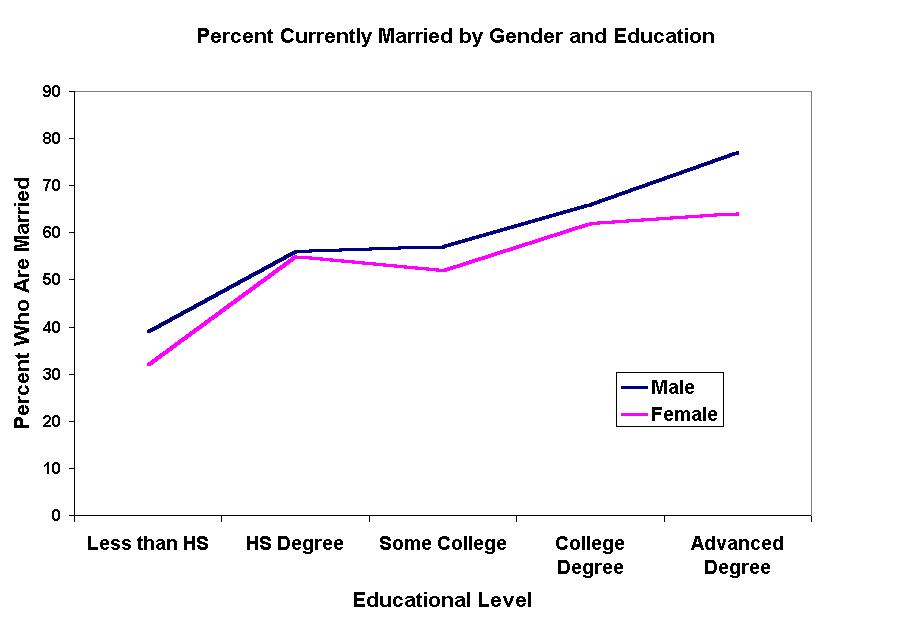
Consider the line graph or percentage polygon below that shows the relationship between educational level and marital status = currently married in the Current Population Survey August 2000 data.
Clearly the percent who are married rises monotonically with each educational level.
Notice how the relationship continuously rises for men, so that men with an advanced degree are the most likely to be married. However, see how the relationship for women "plateaus" at the bauccalaureate level. Women with advanced degrees do not have any apparent advantage over women with B.A. degrees in getting (or staying) married.
Thus, the relationship between marital status and educational level IS DIFFERENT for women and men. This is an interaction effect because the relationship between two variables is specific to a particular condition (i.e., value) of a third variable, in this case, gender.
There are several different patterns
of interaction effects. The key is that the bivariate
relationship between the original independent and dependent variables is
different in at least one category
of the control variable.
Suppose you are investigating the relationship between educational level and income level. I've made up these data for demonstration purposes, so don't be surprised to see them change radically from table to table.
Your first control variable is "field of
diploma." You examine three values or degree fields: business degree, social
science degree, and physical or biological science degree.
| Group considered | Correlation between educational level and income level (tau-b) |
| All cases combined (original table) |
|
| Business degree only |
|
| Social Science degree only |
|
| Physical/biological science degree only |
|
Notice that the relationship is the WEAKEST for the Business majors and STRONGEST for those in the physical or biological sciences but it is always positive (more education = more money). In fact, the strength of the correlation is almost twice as strong for the physical/biological science major in this example as it is for those with a Business degree.
1. POSSIBLE INTERACTION OUTCOME #1. So the bivariate correlation is in the same direction for all the subgroups (all positive in this example) but STRONGER in some subgroups than in others.
Here is a second
example of possible interaction outcome #1 in which the original correlation
between number of cigarettes smoked daily and life expectancy is negative
both for the total sample and in the subgroups. (I made up these numbers
for illustration purposes, too.)
| Group considered | Correlation between number of daily cigarettes and life expectancy in years (Pearson's r) |
| All cases combined (original table) |
|
| American Whites |
|
| American Blacks |
|
The correlation is negative for both ethnic groups, but much more so for Blacks than for Whites, .i.e., the negative relationship is stronger for Blacks than for Whites.
2. POSSIBLE INTERACTION OUTCOME #2. Another possibility is that the original bivariate correlation disappears in at least one subgroup but is of sizable strength in at least one other subgroup. The correlation in one of the groups may even increase over the original bivariate relationship. This IS an interaction effect BECAUSE YOU ARE COMPARING GROUPS WITHIN CATEGORIES OF YOUR CONTROL VARIABLE.
In my fictictious example below, we examine
the correlation between educational level and income level separately for
women and for men:
| Group considered | Correlation between educational level and income level (tau-b) |
| All cases combined (original table) |
|
| Men only |
|
| Women only |
|
In this second example, once the control variable of gender is introduced, the correlation between educational level and income level totally disappears for women but is of moderate strength for men. The original correlation of all groups combined is misleading because the correlation differs so much across the subgroups.
That's what happened with our third order example of gender/degree/quiz question from the 2014 General Social Survey data.
This is one example of why you need to report the associations separately for each partial table when you have statistical interaction. Often analysts will use one of the correlation coefficients for categorical data, but you can also use the odds-ratio or the ln odds. The original correlation for both sexes combined made it appear that there was one set of results (more education = more money; relationship = weak), but in fact, in this table, those results only held for one group (males).
3. POSSIBLE INTERACTION OUTCOME #3. In yet another form of interaction, the bivariate correlation between the original two variables may be positive in one group but the bivariate correlation between the same two variables is negative in a second group.
In the example below, the correlation between the number of children in a family and family income level is weak and positive for industrial countries (wealthier families can afford to have more children and do so) but the correlation between the number of children in a family and family income level is moderate and negative in less developed countries where high fertility may prevent the family from accumulating wealth.
Once more, it would be extremely misleading
to use the bivariate correlation for all the countries combined because
that correlation is so different depending on which type of country is
examined.
| Group considered | Correlation between number
of kids and family income |
| All cases combined (original table) |
|
| Industrialized countries |
|
| Developing countries |
|
Interaction effects can occur with ANY
level of correlation coefficient: nominal, ordinal or interval-ratio. However,
differences of direction can only occur with ordinal or interval-ratio
correlation coefficients because these are the only ones that have
a direction.
 |
OVERVIEW |
|
|
This page created with Netscape
Composer
Susan Carol Losh
January 25 2017