News
Reduced air pollution has improved forest health
March 2014
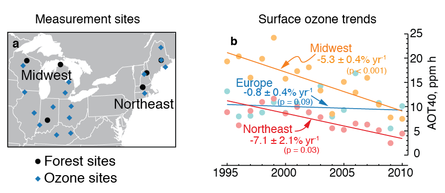
Ozone air pollution harms people and plants. Worldwide, exposure to ozone causes about 700,000 excess deaths each year, as well as impaired breathing, asthma attacks, and reduced crop yields. Changes in vehicle and industrial emissions in the United States required by the Clean Air Act have improved surface ozone air quality significantly in many urban and rural regions. In a recent letter to Nature, I show that these trends of falling ozone help explain some changes in the way forests use water that have been observed, but previously not fully explained. Trees take carbon dioxide from the atmosphere in order to photosynthesize sugars and biomass, but lose water through transpiration in the process. The ratio of carbon dioxide gained to water lost is water-use efficiency. Long-term measurements in many forests in North America and Europe have revealed that forests have increased their water-use efficiency over the last 20 years. Rising carbon dioxide levels in the atmosphere (due to fossil fuel use and deforestation) explain part of the water-use trend, but not all of it. Using empirical relationships between ozone and water use in controlled experiments on many tree species, I show that the ozone trends explain a significant part of the water-use efficiency trends. These ozone-water interactions should be added to future climate and biosphere models to better understand and predict how air pollution affects climate and the carbon and water cycles. |
 |
|
Figure: At rural sites throughout the Northeastern and Midwestern United States (left) surface ozone (O3) pollution has been falling for the last 15 years. Trees and crops injuries from ozone are related to their cumulative exposure to ozone over a season, which is measured as AOT40 (right). AOT40 has fallen 5% per year in the Midwestern US and 7% per year in the Northeastern US. These ozone trends explain about one-sixth of the trend in water-use efficiency that has been observed at nearby forest sites, which is more than can be explained by other factors. |
For more information:
Improved Methane Global Warming Potential (GWP)
February 2013
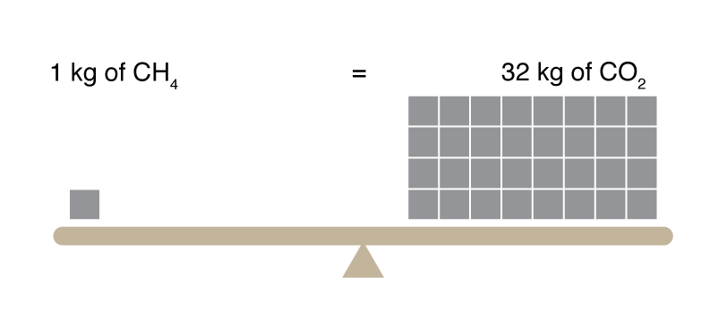
Global Warming Potentials (GWPs) serve as an "exchange rate" among greenhouse gases, enabling emitters to compare the climate benefits of reducing emissions of different gases, such as carbon dioxide (CO2) or methane (CH4). The methane GWP is defined as the total radiative forcing (i.e. heating) over 100 years (or another time horizon) caused by emitting methane, compared to emitting an equal amount of CO2. Since methane is a precursor of ozone and stratospheric water vapor, both of which are greenhouse gases, the methane GWP customarily includes the radiative forcing caused by these decay products. Our analysis suggests that methane breakdown in the atmosphere produces more ozone and more radiative forcing than previously recognized, with most of the additional ozone residing in the stratosphere. New data also revise the methane lifetime upwards (9.1 yr). Taken together, we calculate the methane GWP to be 32, which is 25% larger than past assessments. This high GWP implies that methane emissions are more harmful to the climate than previously thought, but also that reducing those emissions will have greater benefits. Our full analysis of atmospheric methane lifetime, future abundances, and GWP is published in Atmospheric Chemistry and Physics. |
 |
|
Figure: GWP provides a basis for comparing climate heating caused by different greenhouse gases that have different absorbances (heat-trapping ability) and atmospheric lifetimes. Our work suggests that the methane GWP (100 yr) is 32, significantly larger than the value of 25 that that was recommended by the Intergovernmental Panel on Climate Change (2007). |
For more information:
Methane projections for the 21st Century
August 2012
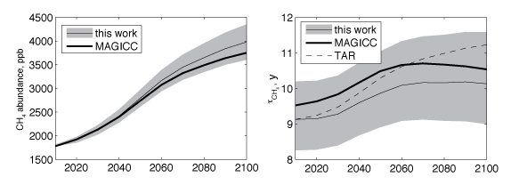
In a new paper in Atmospheric Chemistry and Physics Discussions, we present a new method for predicting atmospheric methane concentrations along any socioeconomic emission scenario. We use a simple and fast modeling approach that accounts for chemistry-climate interactions, including their uncertainties. Since rising greenhouse gas abundances are the main cause of recent climate change and methane is one of the most important greenhouse gases, these results will impact the predicted climate evolution in the 21st century. |
 |
|
Figure:Projected future atmospheric methane abundance (left) and lifetime in the atmosphere (right) in the RCP 8.5 socioeconomic climate and emission scenario. Projected uncertainty (shaded) accounts for uncertainty in the present-day budget, emissions, and chemistry-climate effects. We compare our projections to the MAGICC model and the IPCC Third Assessment Report (TAR) model, which do not include uncertainties. |
For more information:
- Holmes, C. D., M. J. Prather, O. A. Søvde, and G. Myhre (2012) Future methane, hydroxyl, and their uncertainties: key climate and emission parameters for future predictions, Atmos. Chem. Phys. Discuss 12, 20931-20974, doi:10.5194/acpd-12-20931-2012.
- Prather, M. J., C. D. Holmes, and J. Hsu (2012) Reactive greenhouse gas scenarios: Systematic exploration of uncertainties and the role of atmospheric chemistry. Geophys. Res. Lett., doi:10.1029/2012GL051440.
New IDL programming tools
June 2012
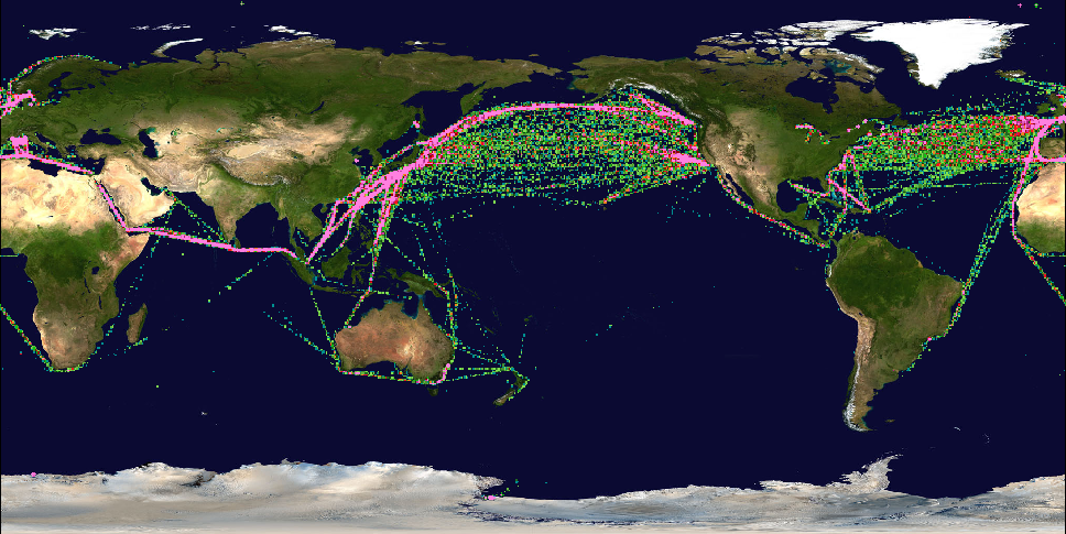
A new library of IDL programs for manipulating netCDF files is now accessible from the Tools page. See NCDF_TOOLS. The programs make reading data and creating netCDF files easy. They are designed especially for geospatial data sets. With WRITE_GEO_NCDF, for example, you can create a netCDF file with 4-D (latitude-longitude-altitude-time) data in just 1 line! |
 |
|
Figure: Global ship traffic in January 2000, shown by intensity of CO emissions. The netCDF file containing the underlying data was created with NCDF_TOOLS. Data from ACCMIP; Graphics by IDV. |
Quick cycling of quicksilver
February 2012
Nature Geoscience (February 2012 issue) contains a "News and Views" column that I wrote about some exciting new airborne measurements of mercury. An article in the same issue, by Seth Lyman and Dan Jaffe, reports the first measurements of elemental and oxidized mercury at high altitudes. Previous modeling work by myself and others suggested that oxidation should be very fast near the tropopause and above. These observations confirm that model result and suggest that particle settling controls the fate of mercury in the upper atmosphere. |
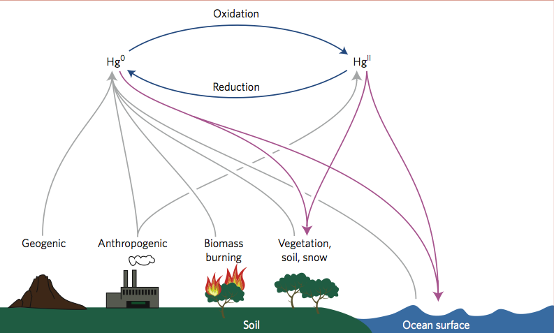
Figure: Atmospheric mercury cycle. Oxidation occurs throughout the atmosphere and new measurements confirm model predictions that it is fastest at high altitudes near the tropopause and above. |
For more information:
- Holmes, C. D. (2012) Nature Geoscience 5, 95-96, doi:10.1038/ngeo1389.
- Lyman, S. N. and D. A. Jaffe (2012) Nature Geoscience 5, 114-117, doi:10.1038/ngeo1353.
- Holmes, C. D., Jacob, D. J., Corbitt, E. S., Mao, J., Yang, X., Talbot, R., and Slemr, F.: Global atmospheric model for mercury including oxidation by bromine atoms, Atmos. Chem. Phys., 10, 12037-12057, doi:10.5194/acpd-10-12037-2010, 2010.
Assessment of climate impact from aviation (and its uncertainties) published in PNAS
July 2011
Aircraft emit nitrogen oxides (NOx) that indirectly warm and cool the climate by increasing tropospheric ozone and decreasing methane, two major greenhouse gases. These opposing effects on climate (quantified as radiative forcing, RF) mostly cancel. Through a survey of prior modeling studies we find that the net steady-state RF from aviation NOx is +4.5 ± 4.5 mW/m2. The 100-year global warming potential (GWP100y) from aviation NOx is thus 52 ± 52. Despite the large relative uncertainty in NOx effects, the climate warming due to aviation CO2 emissions is about 14 times greater, over a 100 year timespan. This work diagnoses the sources of uncertainty in RF with two complementary methods. We find strong correlations among the O3 and CH4 responses to aviation NOx across widely differing models, which is likely caused by differing NOx abundances in each model. Measurements of NOx and other reactive species in the free troposphere could reduce the uncertainty in the climate impact from aviation NOx and other emission sources. |
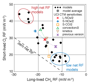 Figure: Steady-state radiative forcing (RF) from O3 and CH4 caused by aviation NOx emissions. RF components are strongly correlated across models, indicating an underlying factor that determines the net climate RF. The UCI CTM reproduces this variability through changes to background NOx. |
For more information:
Global mercury cycle analysis published in ACP
December 2010
We show that atmospheric oxidation of elemental mercury solely by atomic bromine can explain observed global patterns of mercury abundance, gradients, seasonal cycle, and deposition. The model using this oxidation mechanism predicts greater mercury deposition to the high-latitude oceans, where many productive fisheries are located. |
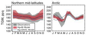
Figure: Mean seasonal cycle of total gaseous mercury (TGM) at 15 sites in the northern hemisphere mid-latitudes and 3 sites in the Arctic. See paper for details. |
For more information: