OVERVIEW

GUIDE 1: INTRODUCTION GUIDE 2: CONSTRUCTING A TABLE GUIDE 3: UNIVARIATE STATISTICS AND DISPLAYS GUIDE 4: BIVARIATE BASICS GUIDE 5: BIVARIATE CORRELATIONS GUIDE 6: MULTIVARIATE CROSSTABULATIONS GUIDE 7: BASIC REGRESSION GUIDE 8: REGRESSION SPECIFICS GUIDE 9: SAMPLING

INTRO STATS READINGS AND ASSIGNMENTS

BIVARIATE DISTRIBUTIONS: REVIEW

We ask three questions about how two variables relate to each other.

1. We ask whether an apparent relationship between two variables in sample data is a SAMPLING ACCIDENT or whether the bivariate relationship is REAL or NON-ZERO. This is about statistical significance or statistical inference.

2.  If (and only if) the apparent bivariate relationship is probably REAL, we ask HOW STRONG the relationship is or the question of substantive significance or effect size.

3.  If the bivariate relationship is REAL and the strength is NONTRIVIAL, we explore the causal nature of the original bivariate relationship. This issue arises the most frequently in data that are observed, naturalistic, or "correlational," as opposed to experimental data. It is easier to tell what is cause and effect in experimental data because the researcher manipulates the intervention or treatment, which is the independent variable(s).

In observational or naturalistic data, we must take the scores on each variable "the way nature gave them to us." For example, societies do not manipulate (directly, anyway) someone's educational level or salary. Gender and birth place are, well, determined at birth.

Thus, the causal tasks for the researcher who works with naturalistic data are more difficult and more challenging than they are for the experimenter. However, as a review of Guide Five, and some preliminary guidelines on causality should assure you, establishing causality in non-experimental data is often possible to do.

For a review of these causal guidelines, click HERE.

REMEMBER, TOO, THAT TERRIFIC AERA BOOK ON CAUSALITY IN OBSERVED DATA. CLICK HERE FOR MORE INFO.
 
 

INTRODUCING A THIRD VARIABLE INTO THE ORIGINAL BIVARIATE RELATIONSHIP

Here are six basic causal possibilities in naturalistic data when a third variable is introduced into the bivariate analysis of your original independent and dependent variables. The posssible causal relationship among these three variables may be, in this order of examination:

• direct (or "extraneous")

• joint

• interactive (moderator, "statistical interaction," conditional, or specified are other terms)

• intervening ("indirect" or "elaborated" or "mediated")

• spurious (an illusion) or

• suppressed

In order to begin to answer this third question, we need to add at least one more variable, which can be used as a "control variable."

This process is sometimes called table elaboration because we are "elaborating" the original relationship between the original independent variable and the original dependent variable by introducing a control variable.
 

A multivariate distribution simultaneously cross-classifies scores on a particular person or case for three (or more) variables.

For example, we might have a multivariate distribution on gender (male/female), marital status (married/not), and presence of children (yes/no). We can simultaneously cross-classify people as one of the following combinations:

• married females with children
• married males with children
• unmarried females with children
• unmarried males with children
• married females without children
• married males without children
• unmarried females without children
• unmarried males without children

Using my example above, with two marital status categories (married versus unmarried), two sexes (female and male), and two parental statuses (with children versus without), this is a 2 X 2 X 2 or 8-cell total table.

We could set up our example this way:

Notice that we have now created TWO separate tables side by side that examine how marital status relates to the presence of children in the home, one for men and one for women.

Although we cannot definitively "prove" causality, our causal inferences will be helped by the introduction of a third or "control variable". In "Table Elaboration," we re-examine the original bivariate relationship separately for each separate category of the control variable. For example, if our control variable were gender, we would  split the sample into men and women (as per the example above) then re-examine the relationship between marital status and the presence of children separately for each sex.

The use of separate or "partial" tables or "subtables" to examine the original relationship between two variables within categories of a third variable (e.g., looking at how marital status influences the presence or absence of children separately for each category of a control variable such as gender) is also called physical control because we have physically separated cases into groups using the control variable.

In Guides 7 and 8, we will contrast physical control with an entity called "statistical control."
 

GLOSSARY REVIEW

I am introducting a lot of new terms here, so you may want to pause, look back over this section, and ensure that you are comfortable with what is meant by the following terms:
 
 

Control Variable Multivariate Distribution Naturalistic Data Partial Table Physical Control Subtable Table Elaboration

 

BIVARIATE QUESTION 3:
WHAT IS THE TRUE CAUSAL STATUS OF THE RELATIONSHIP?

This is the third question we ask about an association between two variables. First, we establish that the relationship is REAL, and at least moderate strength so we know it is not trivial.

We then ask whether the two variables have a "true" causal association, or

Whether the size or direction or form of the relationship between the original two variables differs across categories of a third (or "control" variable), or

Whether a third variable "intervenes" or "mediates" between the original independent and dependent variable, or

Whether a third variable is the actual causal variable for both the original two variables (a spurious relationship).

First, we examine the original bivariate relationship between our independent and dependent variable for the total sample. This means:

• we run the bivariate relationship
• we examine the pattern of percentages
• we assess the statistical significance of the association
• we select the most appropriate bivariate correlation, and
• we examine the selected bivariate correlation coefficient (strength, direction, form, etc.).

Most statistical programs, including DAS and SPSS have a provision to include a "control variable" (DAS) or "layers" (SPSS) in the crosstabulation program.

Third, we examine the correlation between the original independent and dependent variable separately for each "partial table," that is, separately within each value or category of the control variable.

Is the association within each subgroup the same as in the original bivariate table?

Does the association within the "partial tables" differ from the original association? If it is different, how is it different?

Does the association between the original independent and dependent variables differ across categories of the control variable?

Fourth, always remember that our focus is on the original bivariate relationship and what has happened to that bivariate relationship within the subtables. You want to see what has happened to the original correlation once you have controlled for a third variable, or taken the third, or control, variable into account.

If the control variable has only two values (say, male or female in this example), we will have three correlations to examine.

• The first correlation is for the entire sample, which is what you have been doing the past few weeks. For example, you would examine the relationship between marital status and parental status for all respondents combined.

• The second correlation would be for males only. You would examine the relationship between marital status and parental status for the male table alone.

• The third correlation would be for the relationship between marital status and parental status only for females.

For a novice, it can be confusing to wind your way among a series of correlations and then to decide how they match up with possible causal explanations. If you follow the order of the sequence below, this can help to simplify matters at least a little.

• 1. direct (or "extraneous")

• 2. joint

• 3. interactive ("statistical interaction," conditional, "moderated," or specified are other terms)

• 4. intervening ("indirect" or "elaborated"  or "mediated")

• 5. spurious (an illusion) or

• 6. suppressed

For this course, we will use the rule of thumb I call the |.10| rule ("the absolute value of .10 rule") .

Admittedly, this is an "eyeball" rule. (That means you look at the patterns in the data without applying some kind of formal test of statistical inference.) Although it is not a good substitute for formal inference tests, it can help you to explore the different patterns that occur in three-way multivariate tables. More advanced techniques do have formal tests of statistical significance.
 

1. DIRECT RELATIONSHIPS

Considering a "direct" (or "extraneous") relationship first, the values for the original correlation and the correlations in the subtables remain nearly the same for the entire sample and both subgroups (within |.10| of each other). This means that adding a third variable to the analysis does not change the original bivariate correlation.

Consider the following example from the August 2000 Current Population Survey that examines the bivariate association between education and the use of email at home for job or money-making purposes (for example, someone who has an online business or who places auction items on eBay).

Here I am ONLY considering the 31,576 valid (weighted) cases who are persons with online access at home. The more education a person has, the more likely they are to use email for commercial purposes at home. However, because men are more likely to be self-employed than women (and more likely to be employed at all), men may use home email for commercial purposes more than women do, so both education and gender may be independent variables. In fact, men are about 3 percent more likely than women to use home email for commercial purposes in this sample.

The lesson from the above is: pay attention to coding issues!! When you have a correlation and the direction appears "backwards," check the coding on your independent and your dependent variable and see if the way that the variables are coded might be the cause of your computer output anomalie.

The correlation for everyone between educational level and home email for commercial use is Tau-b = + 0.11 (remember, I flipped the sign). It is highly statistically significant, p < .01 but of course there are several thousand cases so it is not surprising that we can reliably conclude that the relationship between these two variables is different from zero.

Our H₀: Tau-b = 0
Our alternative, H_A : Tau-b =\= 0

Considering the subgroup correlations between educational level and home email for commercial use, the separate correlations for women and men are each statistically significant. Again, each separate gender partial table has several thousand cases, so this isn't surprising either.

The correlation for men between educational level and home email for commercial use is:

Tau-b = + 0.12

Tau-b = + 0.10

This combination may be a direct relationship. Although the association is very slightly stronger for men than women, all correlations are within |.10| of each other. Our original causal assertions about the bivariate relationship in the total sample still hold for the time being.

Or, to put it slightly differently, "not much is happening" with the addition of a control variable. The correlation between educational level and home email for commercial use, weak as it is, is "robust." It does not change with the addition of the third variable, gender.

How about gender, our control variable? How much impact does gender have on using home email for commercial purposes?

The correlation coefficient (Phi) between gender and using home email for commercial purposes is highly statistically significant. I used Phi because gender is nominal and home email is ordinal (so I can't use an ordinal correlation coefficient here.)

X² ₍₁₎ = 60.24, p < .01

However, the correlation is so VERY weak:  = .04 that it is basically trivial.

Under these circumstances, we say that gender is EXTRANEOUS ("it doesn't really count") in the relationship between educational level and use of home email for business.

Since gender really has virtually no effect on using home email for commercial purposes, I do NOT consider this a "joint" relationship. It is simply extraneous.

Later on, a research analyst might try additional control variables to see if the relationship between "reduc" and home email use for business continues to exist even after other control variables (such as type of occupation) are introduced.

So this is an "extraneous relationship" that meets two criteria:

• (1) The bivariate relationship between the original independent and the original dependent variable stays pretty much the same in the partial tables formed by values of the control variable and doesn't change (the |.10| "eyeball" rule) and

• (2) The relationship between the control variable and the dependent variable is very weak or zero.

Direct (extraneous) effects is the first possibility about what can happen when you re-examine the original bivariate relationship across categories of a third variable.

It's not too "interesting" because nothing much happens to the original bivariate relationship and the control variable turns out not to influence the dependent or response variable.

If BOTH the original independent variable (after controls) AND the control variable influence the dependent variable together, this is called a joint relationship.

This means that the independent variable AND the control variable jointly affect the dependent variable. Consider the effects of both race and educational level on home ownership.

The dependent variable is the percentage of respondents in the Current Population Survey August, 2000 who currently own their own homes. That percent forms each entry in the cells of the following table. There is another dimension NOT represented here, the percent who DO NOT currently own their own home. Thus what you see below is a THREE WAY CROSSTABULATION TABLE  with only one value on the dependent variable represented (remember: own home versus not own home percentages will add to 100% which is how I can present the table below.)

Put slightly differently, if the entire three dimensional table were presented (including own house, yes and no) there would be 20 cells. 5 columns for educational level, 2 rows for race, and 2 layers back for home ownership.

OWN HOUSE = YES group

For example, 68 percent of Whites with less than a high school education own their own homes; the corresponding figure for Blacks is 48 percent. 83 percent of Whites with an advanced degree own their own homes; 70 percent of Blacks at the same educational level do so.

As we examine the combined row and column percents, we can see that both ethnicity (orange row total percents) AND educational levels (yellow column total percents) influence the percentage owning a house. The percent owning a house rises monotonically with education (from 65% for everyone without a high school diploma to 82% for everyone with an advanced degree.)  However, Whites at any educational level are more likely to own a house than Blacks. For each educational level, the race influence holds, narrowing only very slightly at the very highest degree level.

This is an example of a JOINT RELATIONSHIP. BOTH ethnicity AND educational level JOINTLY affect home ownership.

If it at first appears that you have an "extraneous relationship" and not much has happened to the original bivariate relationship, AND the control variable has an effect on the dependent variable:

Be sure to check NEXT to see what happens to the bivariate correlation between THE CONTROL VARIABLE AND THE DEPENDENT VARIABLE. If this stays about the same too, you have a joint relationship.

Notice how all the correlations in the first table below are within |.10| of one another.
 

Group considered	Correlation between educational level and home ownership
All cases combined (original table)	0.115
White	0.108
Black	0.099

All the correlations in the table below (which sees what happens to the bivariate correlation between race and home ownership controlling for educational level) also stay within |.10| of one another and of the original Phi.

Note that the correlation between race and home ownership does seem to get somewhat smaller as we move from High School level to Advanced Degree (i.e., race has less impact as education rises, which we had noticed in the percentage table)--but not SO small that we would have an interaction effect (see the next section).

We conclude that race and educational level JOINTLY INFLUENCE the incidence of home ownership.

Joint relationships are useful to know about. Many events are "overdetermined," that is, several variables contribute to explaining a single dependent variable. It is often valuable to know exactly how many and what these explanatory variables are.
 

Group considered	Correlation between race and home ownership (Phi) I must use  here because race is nominal. Did I need to use  for the correlation between Home Ownership and Degree? What could I have used instead? Why?
All cases combined (original table)	0.166
Less than High School	0.148
High School	0.188
Some College	0.170
College Degree	0.107
Advanced Degree	0.097

3. INTERACTION EFFECTS

IF the relationship is not direct or extraneous, the next thing you will look for is statistical interaction or moderation.

In interaction or moderated effects, the correlation between the original independent and dependent variables IS DIFFERENT OR CHANGES across the subgroups or categories of the third variable. Here's how you can initially examine your data for statistical interaction. Run the original table and the partial tables.

Examine the partial correlations for the two or more subgroups created by the values of the control variable. If the value of the correlation between the original independent and dependent variables changes or differs across the two (or more) subgroups by at least |.10|, you have an interaction effect (alternative names: specification, moderated or conditional relationship). This means that the bivariate relationship is specific to a particular subgroup or conditional on a particular combination of values of the independent, dependent and control variables.

Interaction effects make analysis more complicated. You can no longer make simple, general statements about the relationship between the independent and dependent variable. Instead, you have to "condition" those statements by specifically referring to a particular subgroup (e.g., men or Blacks). However, interaction effects can also make life more interesting, because variables relate to each other in different ways across subgroups.

These complications are why we check for interaction immediately after extraneous or joint effects. If you have a statistical interaction STOP RIGHT THERE. Do NOT consider possible outcomes 4-6 below. These WILL NOT apply if you have statistical interaction effects.

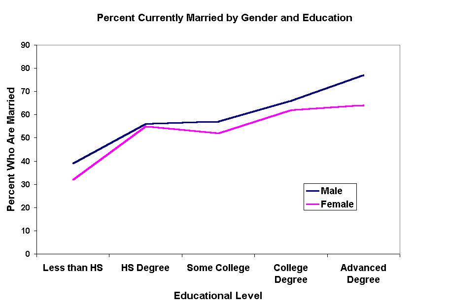
Consider the line graph or percentage polygon below that shows the relationship between educational level and marital status = currently married in the Current Population Survey August 2000 data.

Clearly the percent who are married rises monotonically with each educational level.

[Note: this is a monotonic, rather than a linear, relationship. ASK YOURSELF WHY THIS IS SO.]

Notice how the relationship continuously rises for men, so that men with an advanced degree are the most likely to be married. However, see how the relationship for women "plateaus" at the bauccalaureate level. Women with advanced degrees do not have any apparent advantage over women with B.A. degrees in getting (or staying) married.

Thus, the relationship between marital status and educational level IS DIFFERENT for women and men. This is an interaction or moderated effect (sometimes called a specification or conditional effect). This is because the relationship between two variables is specific to a particular condition (i.e., value) of a third variable, in this case, gender.

There are several different patterns of interaction effects. The key is that the bivariate relationship between the original independent and dependent variables is different in at least one category of the control variable.

Suppose you are investigating the relationship between educational level and income level. I've made up these data for demonstration purposes, so don't be surprised to see them change radically from table to table.

Your first control variable is "field of diploma." You examine three values or degree fields: business degree, social science degree, and physical or biological science degree.
 

Group considered	Correlation between educational level and income level (tau-b)
All cases combined (original table)	+ 0.35
Business degree only	+ 0.25
Social Science degree only	+ 0.36
Physical/biological science degree only	+ 0.47

Notice that the relationship is the WEAKEST for the Business majors and STRONGEST for those in the physical or biological sciences but it is always positive (more education = more money). In fact, the strength of the correlation is almost twice as strong for the physical/biological science major in this example as it is for those with a Business degree.

1. POSSIBLE INTERACTION OUTCOME #1. So the bivariate correlation is in the same direction for all the subgroups (all positive in this example) but STRONGER in some subgroups than in others.

Here is a second example of possible interaction outcome #1 in which the original correlation between number of cigarettes smoked daily and life expectancy is negative both for the total sample and in the subgroups.
 

Group considered	Correlation between number of daily cigarettes and life expectancy in years (Pearson's r)
All cases combined (original table)	- 0.20
American Whites	- 0.15
American Blacks	- 0.35

The correlation is negative for both ethnic groups, but much more so for Blacks than for Whites. (Although these figures were contrived, in fact, cigarette smoking is more lethal for Blacks than for Whites.)

2. POSSIBLE INTERACTION OUTCOME #2. Another possibility is that the original bivariate correlation disappears in at least one subgroup but is of sizable strength in at least one other subgroup. The correlation in one of the groups may even increase over the original bivariate relationship. This IS an interaction effect BECAUSE YOU ARE COMPARING GROUPS WITHIN CATEGORIES OF YOUR CONTROL VARIABLE.

In my fictictious example below, we examine the correlation between educational level and income level separately for women and for men:
 

Group considered	Correlation between educational level and income level (tau-b)
All cases combined (original table)	+ 0.25
Men only	+ 0.40
Women only	+ 0.02

In this second example, once the control variable of gender is introduced, the correlation between educational level and income level totally disappears for women but is of moderate strength for men.

The original correlation of all groups combined is misleading because the correlation differs so much across the subgroups.

This is one example of why you need to report the correlations separately for each partial table when you have statistical interaction. The original correlation for both sexes combined made it appear that there was one set of results (more education = more money; relationship = weak), but in fact, in this table, those results only held for one group (males).

3. POSSIBLE INTERACTION OUTCOME #3. In yet another form of interaction, the bivariate correlation between the original two variables may be positive in one group but the bivariate correlation between the same two variables is negative in a second group.

In the example below, the correlation between the number of children in a family and family income level is weak and positive for industrial countries (wealthier families can afford to have more children and do so) but the correlation between the number of children in a family and family income level is moderate and negative in less developed countries where high fertility may prevent the family from accumulating wealth.

Once more, it would be extremely misleading to use the bivariate correlation for all the countries combined because that correlation is so different depending on which type of country is examined.
 

Group considered	Correlation between number of kids and family income
All cases combined (original table)	- 0.20
Industrialized countries	+ 0.15
Developing countries	- 0.35

Interaction effects can occur with ANY level of correlation coefficient: nominal, ordinal or interval-ratio. However, differences of direction (Type 3) can only occur with ordinal or interval-ratio correlation coefficients because these are the only ones that have a direction.
 

STOP!

If you have interaction effects, do NOT analyze further.

Simply report that you have an interaction effect. Describe how the bivariate correlation is different across the different partial tables or subgroups.

Be sure that there is at least an |.10| difference between the bivariate correlations across the subgroups, as you see in all the fictitious examples above.

Do NOT say "I have a spurious relationship for group one and an extraneous relationship for group two" because that is total nonsense.

In an INTERVENING or MEDIATED RELATIONSHIP, numerically the original bivariate correlation between the independent and the dependent variables becomes much smaller within each category of the control variable.

Directly below is the original correlation between gender and the earth around the sun science question using the 1999 Public Understanding of Science data (n = 1882). The Phi correlation coefficient is 0.18, statistically significant and weak in strength. Below is what happens when we look at the correlation between gender and the science question for each educational level (our control variable) separately:

NOTE: I MADE UP THESE DATA BELOW FOR DEMONSTRATION PURPOSES.
 

Group considered	Correlation between gender and the science question (Phi)
All cases combined (original table)	0.18
High School or less	0.08
Some College	0.07
College Degree	0.07
Advanced Degree	0.08

Look at the correlations from the subtables (marked in YELLOW).

All the correlations marked in yellow are within .10 of one another.

Each one of them is also at least .10 SMALLER than the original correlation (in PURPLE) for all cases combined together. What has hapened is that the original correlation (weak to start with) between gender and the science question "disappeared" in the educational subtables.

(note: alas, this is only for illustration. This did NOT actually happen.)

This is what happens in an "intervening," "mediated," or "explained" relationship:

The original bivariate correlation becomes substantially smaller in each of the subtables. Logically, we say that the original relationship has been "explained" or "mediated" by the control or "intervening" or "mediator" variable which is causally considered the PROXIMATE cause of the dependent variable.

We would diagram this relationship as follows:

Gender      Educational Level     Basic Science Knowledge

Educational level is the most proximate cause of basic science knowledge. But, insofar as it has any effect on education, gender influences education, which, in turn, affects science knowledge.

Notice that the third or CONTROL VARIABLE IS IN THE MIDDLE of the diagram, in between the original independent variable (Gender) and the original dependent variable (Science Knowledge), that is, it INTERVENES OR MEDIATES in between.

The "Head Start" program is another example of an indirect or mediated causal model. Head Start (a vigorous preschool program for USA young children) exerts its greatest influence of children's achievement in the very early grades of school. By high school level, the effect has generally vanished--or has it? By influencing early school achievement--which is the most proximate predictor of later school achievement--Head Start has an INDIRECT CAUSAL EFFECT on high school achievement.

Those who plan to go on to study causal modeling, either through Structural Equation Models or Loglinear models will encounter mediating variables again.
 

NUMERICALLY, spurious relationships look exactly like intervening relationships. The original bivariate relationship becomes substantially smaller in the partial or subtables. This time, I am illustrating with what are often called "causal diagrams" for non-experimental data. In this illustration, size of the fire is positively correlated with the number of fire engines and the fire and with the dollars of fire damage. The initially positive correlation between the number of fire engines and the amount of fire damage in dollars turns to zero within each category of fire size.
 
 

Notice that in this case the "control variable," size of fire, in fact causes both variables: the number of fire engines at the fire and the number of dollars of fire damage.  Instead of being in the middle, the control variable is out to the left with a link to both the original "independent" and the original "dependent" variable. You couldn't put this control variable anywhere else in the diagram than where you see it.

After all, calling out fire engines will not increase the size of the fire, and the size of the fire obviously occurs PRIOR to the amount of fire damage, not subsequent to it.

Statisticians delight in creating such silly examples (remember storks on the roof tops and birth rates in Sweden? Ice cream consumption and assault rates?) to demonstrate that correlation is NOT causation. Just because two variables have a nonzero correlation doesn't mean that one of them causes the other. A third variable could cause both of the original two variables.

However, sometimes the two variables in the original bivariate relationship don't seem silly at all. Researchers try to build a plausible case about why one variable could be the cause of a second. One example is below, from the innocent days of the early 1960s, when parents and teachers alike worried about "drug use": students who smoked [tobacco] cigarettes. A negative (inverse) correlation was found between cigarette smoking and grades. Students who smoked more cigarettes also had lower high school grades.

We'll leave aside the idea that perhaps lower grades drove students to smoke. (Nonsmoking) adults were convinced that nicotine somehow altered brain chemicals to lower concentration and focus (in fact the reverse is true). But it sure seemed reasonable at the time.

Then, by the end of the 1960s, someone else controlled for parental socio-economic status. Students from higher education and income households both smoked considerably less (if at all) and also had higher grades. Students who had parents with lower educational and income both smoked more and had lower grades. The original smoking and grades bivariate correlation dropped to zero within each category of social class.
 
 

Why is this relationship a spurious causal relationship rather than an intervening causal relationship? Because of the location of the control variable. Notice that Student Social Class is off to the far left as the case of both cigarette smoking and school grades. Because the high school student's social class in the study was based on the educational, occupational, and income level of his or her parents, student's original social class could not possibly be caused by either his/her cigarette smoking or the student's grades.
 

If the values of the correlations in the partial or subtables tables are smaller than the correlation for the entire sample (by at least |.10|), you have either an intervening ("indirect" or mediated) relationship OR a spurious relationship.

These are two totally different CAUSAL explanations but NUMERICALLY they look the same. So, how do you know which is which?

• If the control variable goes in the middle in between the original cause and effect, you have an intervening or mediated causal effect. The original independent variable is said to exert an INDIRECT CAUSAL EFFECT on the dependent variable. The control variable is likely to be the MOST PROXIMATE CAUSE of the dependent variable.

• If the control variable is the cause for both the original independent and dependent variable, you have a spurious relationship: the original relationship was an illusion. It "looked real" but was a numeric artifact. It occurred only because the control variable caused both the original "independent" (which was really a dependent variable too in a sense) and the "dependent" variables. In the diagram, the control variable would be to the far left as a cause of both the original independent and the original dependent variables.

Only logic and the position of the third variable will help you answer this question.

Review the section on causal rules to get some hints about the causal location of the third or control variable:

CLICK HERE:
 
 

6. FINALLY: RARE BUT INTRIGUING: SUPPRESSED RELATIONSHIPS

In a SUPPRESSED relationship, "nothing" turns into "something."

In a relatively rare occurrence, the correlations in the partial or subtables are actually LARGER than the bivariate correlation between the independent and the dependent variable in the original table.

Suppressor relationships are so rare I am using made-up data below, just to illustrate what happens. Notice that:

• The correlations separately for women and men are within |.10| of each other (so you don't have an interaction effect).
• Each correlation separately for women and men (.52 and .47) is larger than the original bivariate correlation for both sexes combined by |.10|.

Group considered	Correlation between educational level and income level (-b)
All cases combined (original table)	0.35
Men	0.47
Women	0.52

Suppressor effects tend to happen when there are unusual patterns of negative and positive correlation coefficients among the three variables.

One reason why these are rare in research reports is because supressor effects can happen when the original bivariate coefficient is about zero. The researcher concludes that s/he has nothing going on and doesn't investigate further unless there is some kind of compelling conceptual reason. Sometimes supressor effects emerge almost by accident during multivariate analysis with several independent variables.
 

READINGS AND ASSIGNMENTS

OVERVIEW

Susan Carol Losh October 18, 2004
Revised January 15 2009
This page was built with Netscape Composer